Dynamic Integrated foreCast (DICast®) System
The Dynamic Integrated foreCast (DICast®) system is tasked with ingesting meteorological data (observations, models, statistical data, climate data, etc.) and producing meteorological forecasts at user defined forecast sites and forecast lead times. In order to achieve this goal, DICast® generates independent forecasts from each of the data sources using a variety of forecasting techniques. A single consensus forecast from the set of individual forecasts is generated at each user-defined forecast site based on a processing method that takes into account the recent skill of each forecast module.
DICast® is a licensed technology of UCAR.
History
The DICast® system was first developed at NCAR in the Fall of 1998 with the goal of generating completely automated, timely, accurate forecasts out to ten days at thousands of international locations. Potential applications of this system include the transportation systems, precision agriculture, and general public-oriented forecasts. See the Operations tab for other future applications of this technology.
The DICast® system ingests data from multiple sources and applies automated forecasting techniques to each data source. Each of these forecast modules produces an "independent" forecast. The forecast skill is then improved using a fuzzy logic scheme to combine the individual forecasts.
Over the years, the numerical weather prediction (NWP) model data used by the system has evolved in response to changes to those models and appearance of new ones. The system is currently capable of using all of the US National Weather Service (NWS) modeling suite (GFS, NAM, RAP, HRRR, ensembles of GFS and CMC) as well as MOS guidance (MEX, MET, MAV, LAMP), European Forecast Center's ECMWF, the UKMET model, Environment Canada's GEM model and the Australian Bureau of Meteorology's ACCESS model. Other models such as high-resolution customized versions of WRF can be added based on the user requirements.
The system is designed to generate forecasts of standard meteorological parameters at a set of user configured locations for each forecast lead time. Forecast extent, forecast interval and update frequency are configurable but generally match the input NWP model temporal parameters. Individual module forecasts are combined using a weighted sum. The weights used in the combination are adjusted daily to reflect the recent performance of the forecast modules.
Future Applications And Development
Future Applications for DICast® Technology
The DICast® system was developed for specific applications in the area of public forecasting; however, the basic technology has many potential applications in the future.
- Spot forecasts for wildland fire support – The DICast® system could be used as a forecast engine for providing temperature, relative humidity, precipitation and wind forecasts at fire weather observation sites that are used as input to the National Fire Danger Rating System.
- Track buckling and separation – The DICast® system could be used to provide air and track temperature forecasts for the railroad industry to be ingested into decision support systems that flag sections of track that are susceptible to buckling and separation due to extreme cold or heat, or rapid changes in temperature.
- Military test range support – The DICast® system could be used to provide surface and upper air forecasts of wind, temperature, precipitation, cloud cover and relative humidity for specified points within military test ranges.
- Hurricane landfall conditions – The DICast® system could be used to provide forecasts for wind, precipitation and storm surge at specified locations along coastlines as a hurricane approaches the coast and makes landfall.
- Marine operations – The DICast® system could be used to provide forecasts for marine buoy and oil rig locations for supporting fishing, recreational boating and commercial marine operations.
- Road Weather – The DICast® technology has been reapplied and configured to generate weather forecasts along specific highway routes as part of the Federal Highway Administrations' winter road Maintenance Decision Support System (MDSS) Project.
- Energy – Because of its ability to tune itself based on local observations, DICast® has proven that it is capable of producing a more accurate forecast than any individual input. This skill can be converted to a significant financial benefit by those responsible for predicting energy demands. The energy industry has expressed a lot of interest in DICast®, particularly for electrical power load forecasting.
Future Development for DICast® Technology
The DICast® system is in a continuous state of development so that it can adapt to new and changing data sources as well as utilize new algorithms. Some of the currently planned major additions include:
- Use the European models (ECMWF, UK Met Office)
- Use NWS digital forecasts
- Create probabilistic forecasts
- Add near-term forecast/obs re-alignment (forward error correction)
Performance
Performance Stats
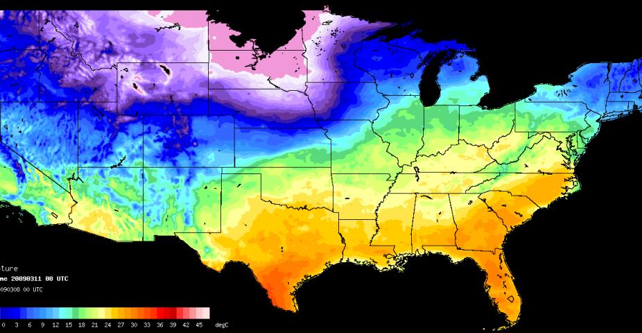
T = Temperature
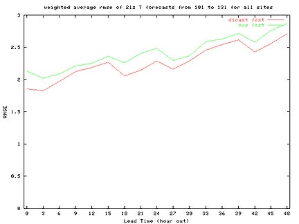
Example of RMSE T-Plot
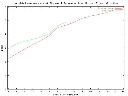
Example of RMSE Max T-Plot
Core Forecasts
The DICast® system generates point forecasts for user–defined locations (e.g., cities, at observation sites, locations along the highway system, agricultural fields, etc.). At observational sites, forecast parameter tuning based on past performance helps improve the forecasts. This class of sites is called core forecast sites. Forecasts at non–core sites are derived from forecasts at core sites.
The numerical weather model data used by DICast® has three–hourly resolution. Since the system is primarily model data driven, forecasts are initially generated at three–hour intervals. These times are called the core forecast lead times.

DICast® Forecast Modules
DICast® creates several independent forecast estimates. Each forecast module attempts to create the best forecast it can by applying a specific forecast technique to its input data set. Each DICast® forecast module uses one of three basic techniques to generate forecasts. They are:
- Dynamic Model Output Statistics (DMOS)
- Interpolation of NWS MOS site forecasts
- Semi-static techniques
Each forecast module produces an identically formatted output file. No forecast module is dependent on another forecast module. That is, no forecast module's output is used as input to another forecast module.
Dynamic MOS forecast modules
The Dynamic MOS (DMOS) forecast modules are a dynamic variation of the traditional NWS MOS procedures. DMOS, like traditional MOS, finds relationships between model output data and observations using linear regression methods. However, while MOS equations are calculated using many years of data, DMOS uses only the last 3 months (configurable) of data. New regression equations are re-calculated once per week.
The DMOS technique has several advantages over traditional MOS. The reliance on only a short history allows DMOS equations to be calculated and DMOS forecasts generated for newly ingested models or models that are changing due to enhancements. Traditional MOS equation generation would require the model to be stable (no changes) for several years. Also, the MOS equations are calculated painstakingly with a large human quality control effort. This makes it difficult to add MOS equations for a new set of forecast sites. DMOS forecasts can be made at these sites immediately provided they have an observational history of at least three months (configurable).
A disadvantage of DMOS is that the equations it produces are less stable than MOS equations. For this reason, quality control checks must be put into place to assure that the equations produced will not create nonsensical outlier forecasts.
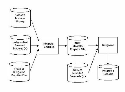
The DMOS subsystem applied to any model has three components:
- Regressor calculation
- Empirical Relationships Generator
- Forecast Generator
The interaction of these three components is illustrated below:

Regressor Calculation
Regressors are variables extracted or derived from model data, which is likely to have a relationship to one of the output forecast variables. These regressors are calculated at each forecast site for each forecast lead-time. About 2/3 of the regressors are variables directly extracted from the model data. Other regressors are derived by combining several variables to estimate meteorological data not explicitly predicted by the models.
Since the forecast sites are rarely at model grid points, interpolation techniques are used to generate forecasts at the forecast sites. This requires an understanding of the projection of the model grid and the terrain assumptions used in each model. As some of the regressors are estimates of meteorological variables at the earth's surface, correcting for the simplified terrain used by the model is important and varies from model to model. The regressors from one model run are all stored in one file. The regressor files are put into a regressor history that the DMOS empirics process uses to calculate regression equations.
DMOS Empirical Relationships Generator
The DMOS Empirical Relationships Generator attempts to find relationships between the regressors and the observations at forecast sites. It does this using a linear regression technique. There are tradeoffs involved in determining the best regression equation. The goodness of fit measure of a regression equation is called its r–squared value. Typically, adding more regressors to an equation increases the r–squared value. However, this also increases the variance of the output forecasts since more regressors are included that do not have a strong relationship to the predictand. Therefore, the desired set of regressors has most of the information leading to a good prediction and does not contain noisy regressors.
Equations that do not have a sufficiently high r–squared value are replaced with a default equation. This default equation is a predefined combination of regressors defined by a meteorologist. A default equation is an attempt to generically replicate a meteorologist's logic in coming up with a forecast. Special, usually derived regressors have been developed for this specific purpose. These default equations generally do not produce the erroneous forecasts that a low r–squared equation might.
This best combination of regressors will vary from site to site, between forecast lead times, and clearly will be different for each forecast variable. The relationships will also vary from season to season and from model to model. The empirics generator is run once per week for each model to find the equations which best fit the most recent data. These equations are stored in a DMOS empirics file and used later by the DMOS forecast generator.
DMOS Forecast Generator
The DMOS Forecast Generator applies the empirical relationships generated by the DMOS Empirical Relationships Generator to the most recent regressors. This generates the DMOS forecast. The relationships between regressors that have done well at predicting the observations recently are used again on today's regressor data to make a DMOS forecast. If any of the regressors that appear in a regression equation are missing, a missing forecast is generated.
NWS MOS Forecast Modules
These forecast modules are based on the MOS products generated by the National Weather Service. The MOS data consist of point forecasts at sites chosen by the NWS. The set of MOS sites is usually a subset of the entire forecast site list. For sites included in any particular NWS MOS forecast, the forecast module tries to reproduce the exact forecast. Where variables are explicitly forecast in the MOS product, they are simply copied. Otherwise, if reasonable, the forecast variable is derived from the MOS data. For some variables, no derivation is reasonable and these variables are left as missing data. If the forecast lead times of the MOS product do not match the system forecast times, the forecast module makes an interpolated forecast where possible.
For many forecast sites no explicit MOS forecasts exist. Forecasts for these sites are generated by interpolation techniques. The interpolated forecasts are generated using the forecasts generated at the MOS sites. No satisfactory interpolation technique has been found that works well for all variables in rough terrain. For example, the interpolation of surface winds in the mountains does not work well using any known technique.
Semi–Static Forecasts
Two forecast modules are called semi–static in that their forecasts depend only on historical data, not on any predictive forecast model. These two are the climatology and persistence forecast modules. These modules look at the past weather over different time ranges and base their forecast on the average weather seen. The climatology forecast module uses data from up to the last 30 years. Monthly averages of the forecast variables have been computed and stored in a climatology file. These monthly climatological values are interpolated to the forecast date. The persistence forecast module averages the observations of the variables seen in recent days to come up with its forecast. The persistence and climatology forecast modules have more effect on the forecasts for longer–term forecasts periods (> 72 hours).
FORECAST INTEGRATION
Integration Overview
The DICast® forecast modules each generate as complete a forecast as possible. This includes a forecast for every forecast variable at every forecast site for every forecast lead time. These independent forecast estimates are combined by the integrator to generate one final consensus forecast. Numerous combination techniques have been developed. Investigation has led to a decision to use an enhanced Widrow–Hoff learning method. This method creates its final forecast using a weighted average of the individual module forecasts. The weights are modified daily by nudging the weights in the gradient direction of the error in weight space. The effect of this is that forecast modules that have been performing well for a particular forecast (variable, site, and lead time) get more weight and the poorly performing modules get less weight. Note that different weight vectors exist for every forecast generation time due to differing latencies in the input data sets. The interaction of components of the integrator is illustrated in the figure below.
Integrator Empirics
This DICast® process runs once per day and updates all the weights based on the performance of the various forecast modules. It reads the observations from the previous day and compares the forecast modules' output that predicted those observations. For each forecast, the errors are computed and the gradient vector in weight space is computed. A step proportional to the size of the combined error is taken in that gradient direction to compute the new weights.
Integrator
The integrator creates a final forecast by making a bias-corrected confidence–weighted sum of the individual module forecasts. It reads the forecasts from the forecast module output files, the weights from the integrator empirics file, performs its calculations, and stores its results.
Non-verifiable Data Extractor
The DICast® forecasting techniques described above only apply to core forecast variables. These are variables that are regularly measured and reported in meteorological observation data. The DMOS forecast modules and the integrator both require specific observations to tune themselves. The weights used in the combination are pre determined by a meteorologist familiar with the models and stored in a configuration file. The model variables to be combined have been extracted by the DMOS regressor calculation process and stored in a regressor file. The Non–Verifiable Data (NVD) extractor reads in the appropriate models' regressor files along with the weight configuration file before creating its weighted combination output.
Post-processor
The post–processor provides a variety of processing options to merge the integrator's forecasts and the NVD forecasts. It attempts also to remove ridiculous forecasts, derive other forecast variables, and spatially and temporally interpolate the forecasts to non–core forecast sites.
Quality control measures are applied to the integrator's output to ensure that no forecasts are well beyond reasonable ranges. Forecast values near the limits are returned to the bounding values. For example, forecasts of 101% probability of precipitation are turned into forecasts of 100%. Forecasts well beyond the bounds are replaced with a missing data flag.
Forecast variables required by users are derived from the core set of MDSS forecast variables. For example, relative humidity is derived from temperature and dew point temperature. The output of the integrator contains only forecasts for core forecast sites. Forecasts at the non–core sites are generated by spatial interpolation from the core sites' forecasts. Temporal interpolation of the three–hourly forecasts to one hour is used to generate the desired final forecast temporal resolution.
Contact
Please direct questions/comments about this page to:
Jeremy Sauer
Software Engineer III